Using Double DQN to Land a Spaceship

One of the most interesting assignments that I worked on in Georgia Tech CS Masters was trying to land a spaceship! In this post, I will document my approach and the results from this journey.

1. About

In LunarLander-V2, the goal is to be able to land the spaceship/lander within the landing pad with zero speed. An agent is able to read the environment states and decide on an action at every frame to land the spaceship/lander correctly.

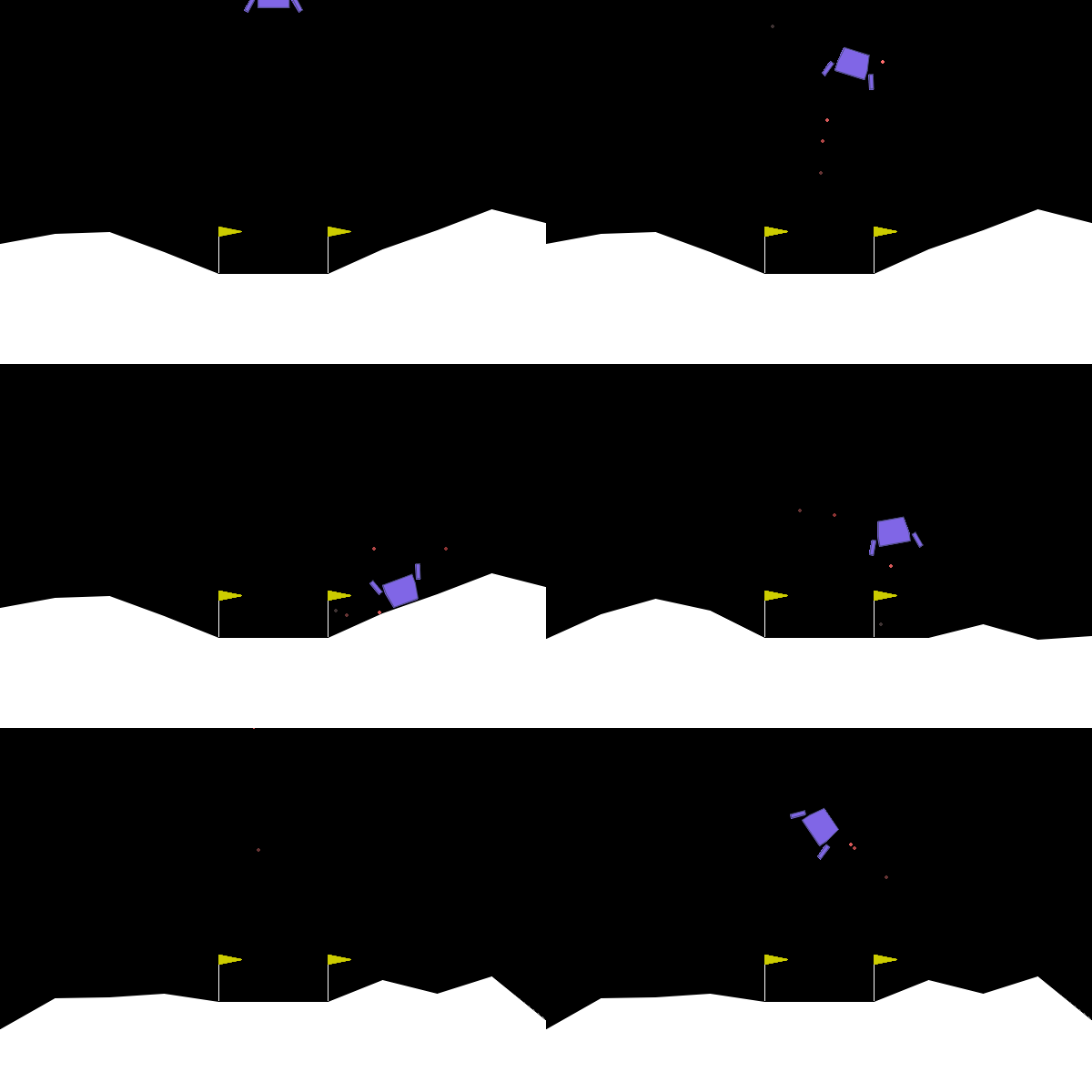
States. State variables are (1) $x$ - coordinate of lander, (2) $y$ - coordinate of lander, (3) $v_x$ - horizontal velocity, (4) $v_y$ - vertical velocity, (5) $\theta$ - orientation in space, (6) $v$ - angular velocity, (7) left leg touching ground, (8) right leg touching ground.

Actions. Four discrete actions are available in the environment: (1) do nothing, (2) fire left orientation, (3) fire main engine, and (4) fire right orientation engine.

Rewards. A reward/scoring system is designed to reinforce positive and negative actions/outcomes in order for an agent to learn. An agent scores points when: (1) the lander moves closer to the landing pad, (2) each leg is rewarded for touching ground +10, and (3) lander comes to rest +100 points. An agent loses points when: (1) lander moves away from the landing pad, (2) lander fires the main engine on each frame -0.3 points, or (3) lander crashes -100 points. The episode ends either when the lander crashes or when it comes to rest.

The spaceship starts at the top of the screen and the landing pad is always at coordinate (0,0). The problem is considered solved when an average score of 200 points in the last 100 episodes is achieved.

2. Approach

Initially, I chose to use DQN as it seems simple enough, yet sufficient for solving an environment with discrete action space such as this. However, there is one paper intrigued me on trying out something different, and that is the Double DQN by Hado van Hasselt (2015).

Pitfalls of DQN. The main issue with Deep Q-Networks (DQN) is their tendency to overestimate action values due to the use of the maximum Q-value for action selection and evaluation, leading to suboptimal policies. Thus, DQNs can experience training instability because of correlations in sequential observations and the non-stationarity of data distributions during learning.

Double DQN. This is where Double DQN comes in. It is exactly designed to address this overestimation bias. Double DQN mitigates this issue by decoupling the action selection and evaluation processes. Specifically, it uses the online network to select the best action and the target network to evaluate the value of that action. This separation reduces the likelihood of overestimation, leading to more accurate value estimates and improved learning stability.

With the Double DQN architecture, we update the weights on the main model every step and only update the target network weights after every $n$ steps, which we can tune as a hyperparameter. This update can be a:

• Hard update. Copying the primary network's weights to the target network, or
• Soft update. Updating the target network's weights towards the primary network's weights using a factor $\tau$

In this study, I chose to use soft updates since I found it to stablize and learn better. The diagram below shows the DQN architecture and how the Double DQN is trained and updated:

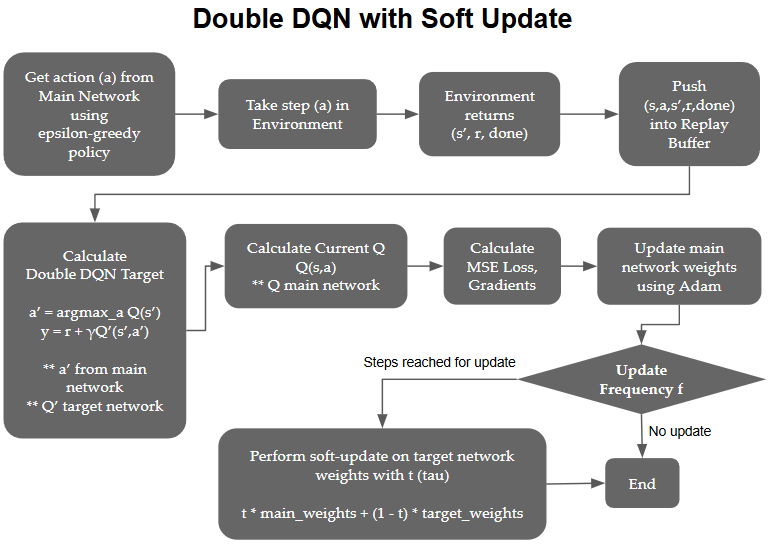
Fig 1. Soft Update of Main and Target Network Weights

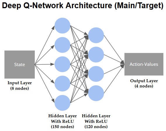
Fig 2. Double DQN Main and Target NN Architecture

To put it to a simple test for comparing the performance of DQN vs. Double DQN, I've used the same hyperparameters for both models and tested to see how long it takes for both models to converge. Here are the results of the comparison:

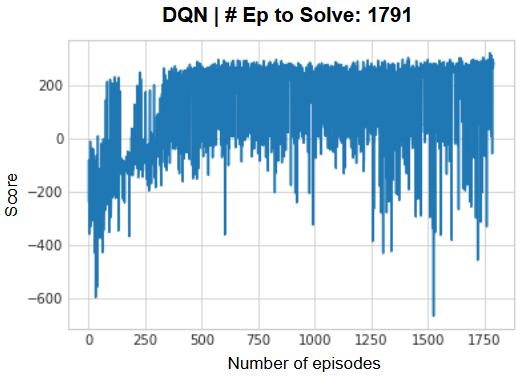
Fig 3a. DQN Initial Results

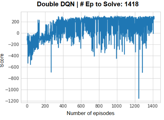
Fig 3b. Double DQN Initial Results

From the initial results, we can see that DQN takes 1,791 episodes to solve the environment, while Double DQN solves in 1,418 episodes. Double DQN converges significantly faster than DQN, showcasing improved efficiency due to its ability to address the overestimation bias. From the DQN chart, it exhibits higher reward variance, likely a result of overestimating Q-values during training. While in the Double DQN chart, it displays more stable learning trajectories, with lower variance in rewards across episodes. The reduced variance in Double DQN ensures more consistent and predictable performance improvements over episodes.

3. Tuning Hyperparameters

Next, I also explored tuning various hyperparameters. The graphs below are a summary of the effects of choosing certain values for different hyperparameters:

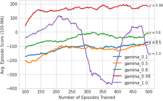
Fig 4a. Effect of Gamma $\gamma$

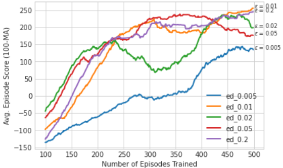
Fig 4b. Effect of Epsilon $\epsilon$

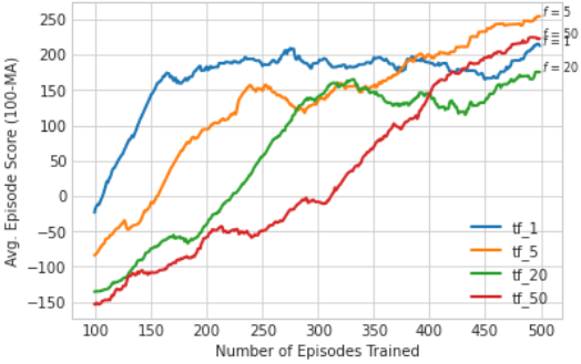
Fig 4c. Effect of Update Frequency $f$

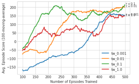
Fig 4d. Effect of Soft Update Tau $\tau$

Gamma $\gamma$. The choice of the discount factor, gamma (γ), significantly affects the learning performance in the LunarLander-V2 environment. A higher gamma value, such as 0.99, emphasizes future rewards and results in the best learning performance by enabling the agent to prioritize long-term goals, like successful landings. In contrast, lower gamma values (e.g., 0.1, 0.5, 0.8) heavily discount future rewards, limiting the agent's ability to associate intermediate actions with eventual success. When γ equals 1.0, future and immediate rewards are treated equally, but this often leads to high variance in learning as the final reward becomes overly emphasized, diluting the importance of intermediate steering actions. Overall, a gamma value of 0.99 strikes an effective balance between immediate and long-term rewards, leading to stable and effective learning.

Epsilon Decay $\epsilon$. The epsilon decay rate plays a critical role in balancing exploration and exploitation during training. Lower decay values (e.g., 0.005) result in excessive exploration, causing the agent to spend more time trying random actions and achieving lower average scores. Moderate decay rates (e.g., 0.01, 0.02, 0.05) lead to better performance, as the agent transitions smoothly from exploration to exploitation. A higher decay rate (e.g., 0.5) accelerates the shift towards exploitation, yielding faster learning but slightly lower long-term stability. The optimal decay rate identified in the study is 0.2, which strikes a good balance between efficient learning and stable performance, allowing the agent to explore effectively while capitalizing on learned strategies.

Target Network Update Frequency $f$. This significantly impacts learning performance in the LunarLander-V2 environment. A low update frequency (e.g. f=1) leads to frequent updates, resulting in higher variance in Q-value estimates and unstable learning. Conversely, a high update frequency (e.g. f=20,50) reduces variance but delays the propagation of learned updates, slowing the learning process. The optimal frequency (f=5) balances these trade-offs, providing sufficient stability in target values while maintaining efficient learning. This value ensures a consistent flow of updated Q-values without excessive delays or fluctuations, leading to improved learning performance.

Tau $\tau$. The soft update parameter $\tau$ determines the rate at which the target network incorporates updates from the primary network. Small values of $\tau$ (e.g. τ=0.001,0.01) result in gradual updates, promoting stable learning and reducing the impact of noise and outliers. However, very low $\tau$ can slow the learning process. Larger values (e.g. τ=0.1) accelerate updates, but may introduce instability due to greater sensitivity to transient fluctuations. The optimal value identified in the study is 0.01, which offers a balance between stability and learning speed, leading to consistent and reliable performance improvements.

4. Final Results

So finally, after all that tuning and setting our best hyperparameters, here's our final agent solving the Lunar Lander in 206 episodes.

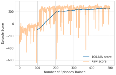
Fig 5. Double DQN Final Results

5. Summary

In summary, here I've demonstrated the use of Double DQN for simple task of landing our million-dollar spaceship on the moon (in 2d game environment), and showed how DQN has the ability to mitigate the overestimation of Q-values, by using a main and target network.

I've also studied the effects of different choices of hyperparameters:

• Discount Factor (γ): A high value (0.99) improved learning by emphasizing long-term rewards.
• Epsilon Decay (ε_decay): A moderate decay rate (0.2) balanced exploration and exploitation effectively.
• Target Neural Network Update Frequency (f): An update frequency of 5 minimized Q-value variance without delaying learning.
• Soft Update Weight (τ): A small weight (0.01) stabilized learning by gradually updating the target network.

Thanks for reading and I hope you enjoyed this post!

References: