- Published on
Estimating Price Elasticity using Double ML
- Authors

- Name
- Kenneth Lim
In my previous post, I demonstrated how machine learning suffers from regularization bias when estimating causal effects. In this post, I will apply the DoubleML framework by Bach et al. (2021) to address this.
Before, I start I would like to mention one of my favorite books in this field: "Casual Inference in Python" by Matheus Facure available on Amazon. It contains a rather comprehensive coverage of causal inference methods, as well as practical applications. Also, do check out his GitBook Causal Inference for the Brave and True as well, which is also very informative and well written along with code.
So now, back to our research to test out DoubleML and see how well it works.
Approach
Similar to the previous post, I will run simulations to generate dataset and estimate the causal effect, but using DoubleML this time. Both causal estimates and prediction accuracy will be compared against OLS model.
Code Implementation
def prepare_dataset(err_std=0.002, seed=0):
    df = generate_dataset(err_std=err_std, seed=seed)
    drop_features = ['M_1', "D_0", "date", "demand", "price", "d_q"]
    return (
        df
        .assign(ln_price=lambda d: np.log(d.price))
        .assign(ln_demand=lambda d: np.log(d.demand))
        .drop(drop_features, axis=1)
    )


def run_ols(dataset, prefix="ols"):
    target = "ln_demand"
    predictors = " + ".join([c for c in dataset.columns if c != target])

    model = smf.ols(f'{target} ~ {predictors}', data=dataset).fit()
    pe_coef = model.params['ln_price']

    yhat = model.predict(dataset)
    rmse = mean_squared_error(dataset.ln_demand, yhat) ** 0.5

    return {f"{prefix}_pe_coef": pe_coef, f"{prefix}_rmse": rmse}


def run_doubleml(dataset, prefix="dml", reg_params={}):
    outcome = "ln_demand"
    treatment = "ln_price"

    X = dataset.drop([outcome, treatment], axis=1)
    T = dataset[treatment]
    y = dataset[outcome]

    outcome_model = LGBMRegressor(verbose=-1, **reg_params)
    treatment_model = LGBMRegressor(verbose=-1, **reg_params)

    y_hat = cross_val_predict(outcome_model, X, y, cv=2)
    T_hat = cross_val_predict(treatment_model, X, T, cv=2)
    df_res = pd.DataFrame({"y_res": y - y_hat, "T_res": T - T_hat})

    model = smf.ols('y_res ~ T_res', data=df_res).fit()
    pe_coef = model.params['T_res']

    yhat_y_res = model.predict(df_res)
    y_hat_final = y_hat + yhat_y_res
    rmse = mean_squared_error(y, y_hat_final) ** 0.5

    return {f"{prefix}_pe_coef": pe_coef, f"{prefix}_rmse": rmse}


results = []

for seed in np.arange(500):
    dataset = prepare_dataset(err_std=0.2, seed=seed)
    ols_result = run_ols(dataset)
    dml_result = run_doubleml(dataset, reg_params={"n_estimators": 300, "max_depth": 6})
    dml2_result = run_doubleml(dataset, prefix="dml2", reg_params={"n_estimators": 200, "max_depth": 4})
    dml3_result = run_doubleml(dataset, prefix="dml3", reg_params={"n_estimators": 50, "max_depth": 2})
    result = {"seed": seed, **ols_result, **dml_result, **dml2_result, **dml3_result}
    results.append(result)

df_result = pd.DataFrame(results)
3. Results and Analysis
And here is the results of using DoubleML, just astonishing:
3.1 Causal Estimates for Price Elasticity

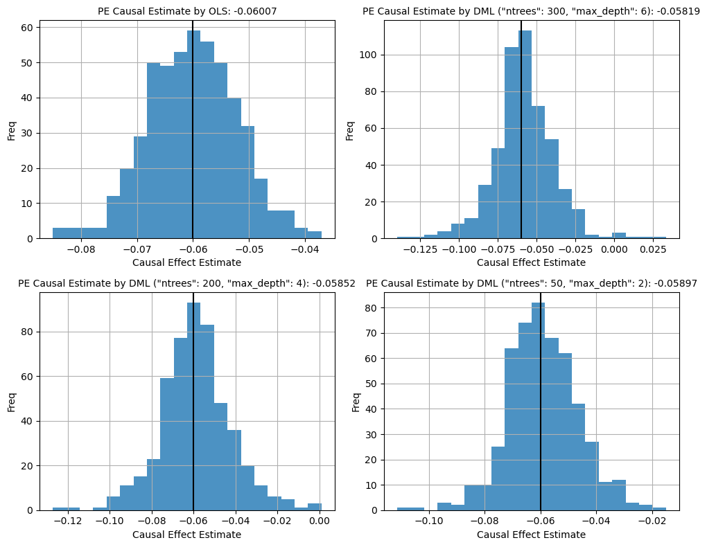
Figure 1. Histogram Plot of Causal Esimates from Simulation
With the DoubleML framework, it is observed that the causal estimate now is very close to the true causal effect value, in contrast to what we had previously using traditional ML. DoubleML has managed to address regularization bias, regardless of the choice of hyperparameters. This allows us to focus on tuning our model to improve prediction accuracy without having to worry too much about having an inaccurate casual estimate of our treatment variable.
3.2 RMSE

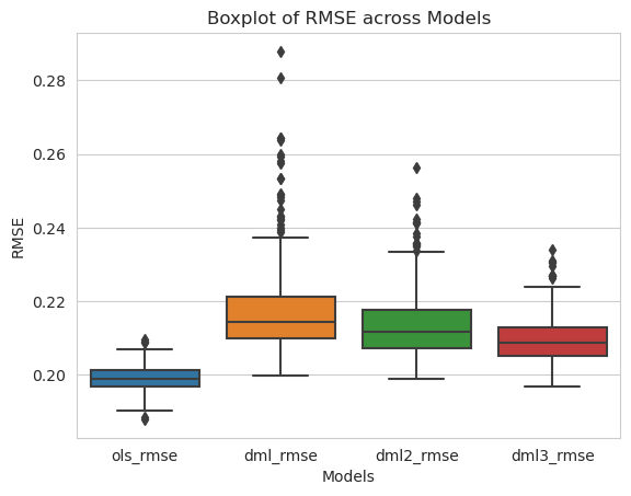
Figure 2. Boxplot of Model RMSEs from Simulation
Despite the improvement in the accuracy of our price elasticity causal estimate, our prediction accuracy here have seem to have suffered, performing even worse than OLS. Remember our synthetic data was generated using linear relations, and definitely OLS Regression is the perfect model here since it encompasses the true process of how the data is generated. Hence, no surprises here as our Gradient Boosting tree does not have the mathematical form to capture the true linear relations.
4. Why it works
DoubleML effectively addresses regularization bias through a process known as orthogonalization, which is closely related to the Frisch-Waugh-Lovell (FWL) theorem.
Frisch-Waugh-Lovell Theorem and Orthogonalization
The FWL theorem states that in a linear regression model, the coefficient of a variable can be obtained by:
- Regressing the dependent variable on the control variables to obtain residuals.
- Regressing the independent variable of interest on the control variables to obtain residuals.
- Regressing the residuals from step 1 on the residuals from step 2 to estimate the coefficient of interest.
This process effectively "partials out" the influence of control variables, isolating the relationship between the independent variable and the dependent variable.
DoubleML
DoubleML extends this idea by using machine learning models to estimate the relationships in steps 1 and 2, allowing for flexible modeling of complex, non-linear relationships without imposing strict parametric forms. The steps in DoubleML are:
- Estimate the outcome model: Predict the outcome variable using covariates to obtain residuals.
- Estimate the treatment model: Predict the treatment variable using covariates to obtain residuals.
- Regress the outcome residuals on the treatment residuals to estimate the causal effect.
DoubleML leverages the principles of the FWL theorem through orthogonalization to effectively address regularization bias, enabling accurate causal inference in complex modeling scenarios.
5. Conclusion
Here, I've shown that Double Machine Learning (DoubleML) framework effectively addresses regularization bias in estimating causal effects.
By employing orthogonalization techniques, DoubleML isolates the treatment effect from nuisance parameters, ensuring that the estimation remains unbiased even when utilizing regularized machine learning models. This approach allows for the flexibility of machine learning in capturing complex, non-linear relationships while maintaining the robustness of causal inference.
Nevertheless, no matter how good ML models are, choosing the right model/algorithm based on understanding the data is still crucial. We have just seen an epsiode of David vs. Goliath (OLS vs. LightGBM) and how David managed to beat Goliath, just because the data force was with him.
Thanks for reading, I hope this post was useful to you in any way. Have a great day!
References: