ML Regularization Bias in Estimating Causal Effects

Machine learning (ML) has revolutionized the way we analyze data, moving beyond predictions to enable causal inference—understanding the cause-and-effect relationships between variables. This capability is particularly valuable in fields like healthcare, economics, and marketing, where determining the impact of an intervention is critical. However, applying ML to causal inference is not without challenges. One prominent issue is regularization bias, which arises when algorithms penalize model complexity to improve generalization. While this bias can reduce overfitting, it may inadvertently distort causal estimates by shrinking coefficients toward zero, leading to underestimation of true causal effects. Addressing this balance between regularization and unbiased causal estimation remains a key focus in advancing ML methodologies for causal inference.

Building on the framework established in the Double Machine Learning (Double ML) by Bach et al. (2021), I will replicate the study to explore the impact of regularization bias and investigate how the degree of regularization relates to the error in causal estimates. Using the data generation function described in the previous post, I will conduct a series of simulations to fit both standard Ordinary Least Squares (OLS) regression models and standard machine learning models.

This study aims to shed light on the trade-offs between regularization, model flexibility, and the accuracy of causal inference, specifically in the context of measuring price elasticity.

1. Approach

A dataset will be generated (using previous generate_dataset function in previous posts) through a controlled simulation using the prepare_dataset function with some noise level err_std. Here, I will be using 0.2 to yield some reasonable variance in our estimate for analysis. Then I will fit both OLS and ML models on the simulated data, with multiple variations of the ML model differing in regularization parameters (from heavy to light regularization). Both models will be using the same set of features.

To extracting the price elasticity coefficient from ML model, I will be regressing a local linear model using ln(price) on the predicted (learned) outputs. The local linear model will then be able to show us what price elasticity coefficient the ML model has learned.

The simluation will be repeated 500 times so we can collect some decent sample of PE estimates for the analysis. In addition, I will also be calculating and RMSE from the models.

2. Code Implementation

The implement is fairly straight-forward with ~50 lines of code:

def prepare_dataset(err_std=0.002, seed=0):
    df = generate_dataset(err_std=err_std, seed=seed)
    drop_features = ['M_1', "D_0", "date", "demand", "price", "d_q"]
    return (
        df
        .assign(ln_price=lambda d: np.log(d.price))
        .assign(ln_demand=lambda d: np.log(d.demand))
        .drop(drop_features, axis=1)
    )


def run_ols(dataset, prefix="ols"):
    target = "ln_demand"
    predictors = " + ".join([c for c in dataset.columns if c != target])

    model = smf.ols(f'{target} ~ {predictors}', data=dataset).fit()
    pe_coef = model.params['ln_price']

    yhat = model.predict(dataset)
    rmse = mean_squared_error(dataset.ln_demand, yhat) ** 0.5

    return {f"{prefix}_pe_coef": pe_coef, f"{prefix}_rmse": rmse}


def run_ml(dataset, prefix="ml", reg_params={}):
    target = "ln_demand"

    X = dataset.drop([target], axis=1)
    y = dataset[target]

    # Ensure our price elasticity constraint is negative
    mono_constraints = [-1 if c == "ln_price" else 0 for c in X.columns]
    ml_model = LGBMRegressor(
        **reg_params,
        monotone_constraints=mono_constraints,
        verbose=0,
    ).fit(X, y)

    yhat = ml_model.predict(X)
    local_dataset = pd.DataFrame({
        "ln_demand": yhat,
        "ln_price": dataset["ln_price"]
    })
    local_model = smf.ols('ln_demand ~ ln_price', data=local_dataset).fit()
    pe_coef = local_model.params['ln_price']
    rmse = mean_squared_error(dataset.ln_demand, yhat) ** 0.5

    return {f"{prefix}_pe_coef": pe_coef, f"{prefix}_rmse": rmse}


results = []

for seed in np.arange(500):
    dataset = prepare_dataset(err_std=0.2, seed=seed)
    ols_result = run_ols(dataset)
    ml_result = run_ml(dataset, reg_params={"n_estimators": 300, "max_depth": 6})
    ml_result_2 = run_ml(dataset, prefix="ml2", reg_params={"n_estimators": 200, "max_depth": 4})
    ml_result_3 = run_ml(dataset, prefix="ml3", reg_params={"n_estimators": 50, "max_depth": 2})
    result = {"seed": seed, **ols_result, **ml_result, **ml_result_2, **ml_result_3}
    results.append(result)

df_result = pd.DataFrame(results)

3. Results and Analysis

And in just about a minute, here's our result:

3.1 Causal Estimates for Price Elasticity

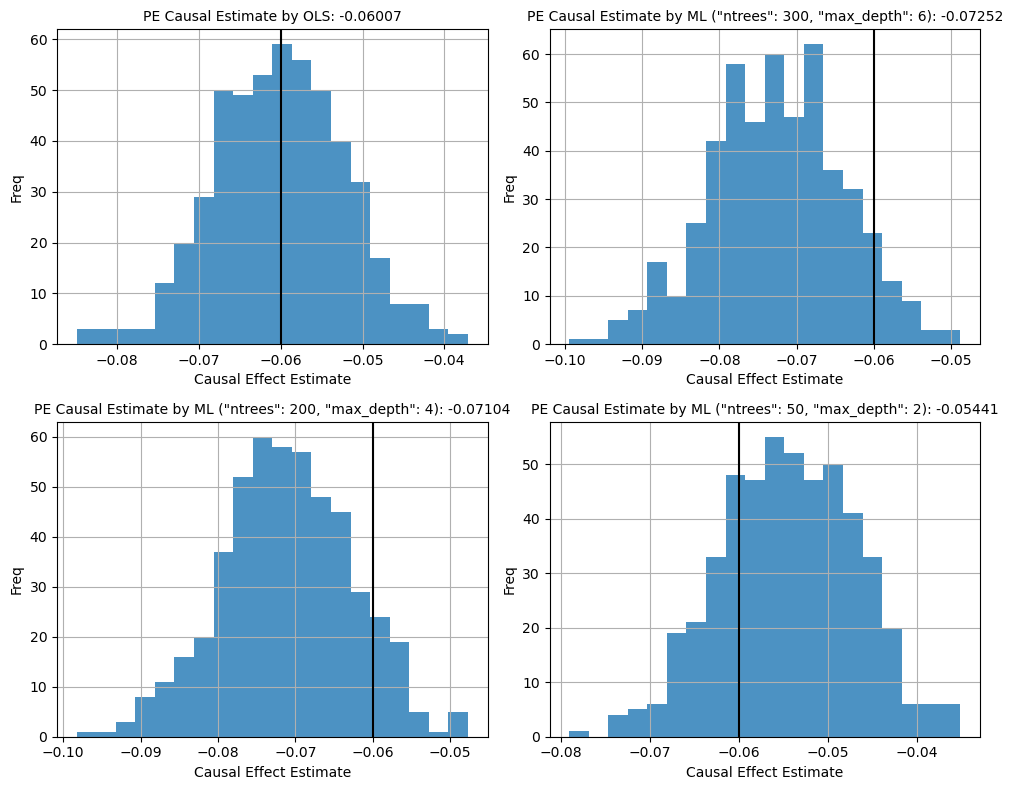
Figure 1. Histogram Plot of Causal Esimates from Simulation

The histograms illustrate the distribution of price elasticity (PE) estimates obtained from 500 simulations for four different models. The true causal effect is denoted by the black vertical line in each plot.

OLS Model. The OLS model produces a tightly centered distribution around its mean estimate (-0.06007), which is really, really close to the true causal effect. OLS works really well here since there's no regularization bias and more importantly, the underlying data was generated using a linear model, hence fitting with OLS works perfectly. In real world, data can come with real potential complexities which a linear model may not suffice.

ML Models The ML model with the strongest regularization produces a distribution centered at -0.05441, which is biased upwards relative to the true causal effect. The model with moderate regularization (bottom left) has estimated an effect closer to the true causal effect. This may suggest a better bias-variance trade-off with less overfitting. The ML model with the strongest regularization (bottom right) yields a much lower estimate of -0.05441, lower than that of the true estimate. Overall, here we can clearly see a demonstration of how regularization has an effect on our causal estimate. Hence, the name Regularization Bias.

3.2 RMSE

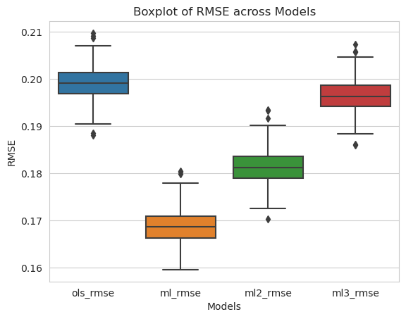
Figure 2. Boxplot of Model RMSEs from Simulation

From the plots above, it is observed that ML model with least regularization has performed the best in RMSE, as expected.

Comparing the accuracy of predictions and causal estimates, we can notice that regularizing ML models is a tricky thing here. There is an apparent trade-off between predictive performance (RMSE) and causal inference accuracy. While reducing regularization can improve RMSE and causal estimate accuracy, excessive reduction in regularization may result in improving RMSE, but reducing the causal estimate accuracy.

4. Conclusion

In summary:

• OLS regression provides stable causal estimates. However, due to its restrictive linear form, it may produce slightly biased estimates and/or may not be sufficient to model higher complexities, resulting in less accurate predictions as well.
• ML models, though can capture higher complexities and be more accurate in predictions, suffer from Regularization Bias. Thus, affecting the accuracy of our causal estimate.

In this post, the ML model functions similarly to an S-Learner in estimating causal relationships, where:

• $X$ excluding ln_price are our covariates, and
• $T$ is our treatment ln_price

Knowing that there will be regulariziation biases, should we still use S-Learner? It depends. While S-Learner has its own shortfalls, S-Learner is still conceptually simpler, computationally cheaper, and can be easier to scale. Fitting a single predictive model that includes both covariates and the treatment variable is easy. It can serve as a baseline model or MVP before investing more. If the accuracy of causal estimate is not that important to you, S-Learner is definitely worth to consider.

Thanks, I hope you enjoyed the read if you've made it this far!

References: