Hierarchical Modeling for Improving Causal Estimate Robustness

In this post, I will be modeling price and cross elasticity with the data generated from the previous post. If you're reading this blog for the first time and would like to check out on my older posts related to pricing, you can view all the posts here.

About the dataset. The dataset is a synthetic time series for three interrelated products, incorporating price elasticity and cross elasticity dynamics. It simulates daily demand over three years, including other components such as trend, seasonality and holidays.

1. Approach

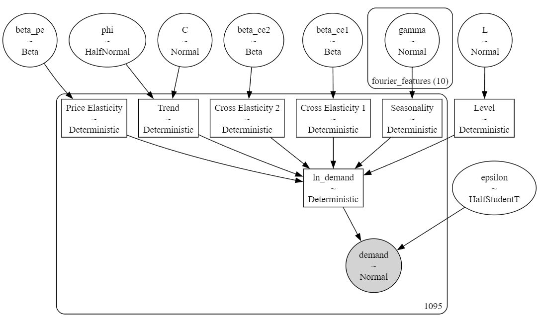
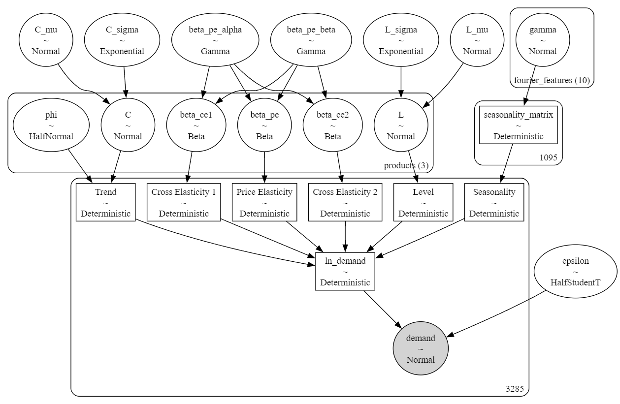
Here I will be exploring modeling with Bayesian regression models. I will (1) build local models to estimate elasticities for each of the three products, and (2) build a single global hierarchical model and estimate elasticities for all products at once. I'll compare and analyze these estimates, then briefly discuss about the results, and finally suggest how we can take that feedback to improve our Bayesian models.

In order to generate more comparable results, I've introduced a relatively high level of noise of err_std = 80, to allow coefficients to be estimated with larger confidence interval for comparison among the methods.

About Bayesian Hierarchical Modeling

Bayesian Hierarchical Modeling is a statistical approach that uses Bayesian inference to analyze data with a multi-level structure. It is particularly useful when the data can be grouped or nested, such as sales data across regions, student performance across schools, or demand across product categories. In this framework:

Hierarchical Structure. Models incorporate both group-level (global) parameters and individual-level (local) parameters, capturing variations within and between groups.
Uncertainty Quantification. Prior beliefs about parameters are combined with observed data to update beliefs (posterior distributions), enabling uncertainty quantification at all levels.
Pooling. By sharing information across groups (partial pooling), the model avoids overfitting and improves robustness, especially for smaller datasets.

Bayesian Hierarchical Models are widely applied in fields like marketing, healthcare, and education for tasks such as demand forecasting, causal inference, and personalized recommendations. They provide flexibility, interpretability, and a principled way for estimating effects and quantifying uncertainty.

2. Code Implementation

Here I'll just dive straight into the final code implementation. The Bayesian Workflow, written in one of my previous posts, is mainly the approach on how I select priors and construct the model gradually.

2.1 Local Models

Figure 1a. Bayesian Regression Model (Local)

def run_local_model(
    t, fourier_features, ln_price, ln_price_s1, ln_price_s2, y_obs
):
    """
    Run a Bayesian Local Model for demand forecasting using PyMC.

    Parameters:
    ----------
    t : ndarray
        Time index representing the progression of time.
    fourier_features : ndarray
        Matrix of Fourier-transformed seasonal components (e.g., sine and cosine terms) for capturing seasonality.
    ln_price : ndarray
        Logarithm of the price of the primary product being modeled.
    ln_price_s1 : ndarray
        Logarithm of the price of substitute product 1, used to model cross-elasticity effects.
    ln_price_s2 : ndarray
        Logarithm of the price of substitute product 2, used to model cross-elasticity effects.
    y_obs : ndarray
        Observed demand data for the primary product.

    Returns:
    -------
    idata_single : arviz.InferenceData
        Inference data object containing posterior samples, prior samples, and posterior predictive checks.
        Can be used for posterior analysis, model diagnostics, and visualization.
    """
    t_norm = (t - t.min()) / (t.max() - t.min())
    coords = {"fourier_features": fourier_features_names}
    with pm.Model(coords=coords) as model_local:
        # Level
        level = pm.Normal("L", mu=0.0, sigma=2.0)
        L = pm.Deterministic("Level", level)

        # Trend
        phi = pm.HalfNormal("phi", sigma=6.0)
        C = pm.Normal("C", mu=0.0, sigma=5.0)
        T = pm.Deterministic("Trend", (C / (1.0 + pm.math.exp(-phi * t_norm))))

        # Seasonality
        gamma = pm.Normal("gamma", mu=0, sigma=0.05, dims="fourier_features")
        S = pm.Deterministic("Seasonality", pm.math.dot(fourier_features, gamma))

        # Price Elasticities
        beta_pe = pm.Beta("beta_pe", alpha=2, beta=5)
        PE = pm.Deterministic("Price Elasticity", -1 * beta_pe * ln_price)

        # Cross Elasticities
        beta_ce1 = pm.Beta("beta_ce1", alpha=2, beta=5)
        beta_ce2 = pm.Beta("beta_ce2", alpha=2, beta=5)
        CE1 = pm.Deterministic("Cross Elasticity 1", beta_ce1 * ln_price_s1)
        CE2 = pm.Deterministic("Cross Elasticity 2", beta_ce2 * ln_price_s2)

        # Linear Component
        ln_demand = pm.Deterministic("ln_demand", L + T + S + PE + CE1 + CE2)

        # Observed data
        epsilon = pm.HalfStudentT("epsilon", sigma=5.0, nu=10)
        pm.Normal("demand", mu=pm.math.exp(ln_demand), sigma=epsilon, observed=y_obs)

        # Sample data
        idata_local = pm.sample(
            chains=4,
            tune=500,
            draws=1000,
            return_inferencedata=True,
            idata_kwargs={"log_likelihood": True},  # Required for az.compare
        )
        pm.sample_posterior_predictive(idata_local, extend_inferencedata=True)

    return idata_local


## Define inputs
y_obs_p1 = df.demand_p1.values / df.demand_p1.values.mean()
y_obs_p2 = df.demand_p2.values / df.demand_p2.values.mean()
y_obs_p3 = df.demand_p3.values / df.demand_p3.values.mean()

ln_price_p1 = np.log(df.price_p1.values)
ln_price_p2 = np.log(df.price_p2.values)
ln_price_p3 = np.log(df.price_p3.values)

t = df.t.values
fourier_features_names = [*[f"cos{i}" for i in np.arange(5) + 1], *[f"sin{i}" for i in np.arange(5) + 1]]
fourier_features = df[fourier_features_names].values

var_names = ["L", "C", "phi", "gamma", "beta_pe", "beta_ce1", "beta_ce2"]


## Fit local models
idata_local_p1 = run_local_model(t, fourier_features, ln_price_p1, ln_price_p2, ln_price_p3, y_obs_p1)
az.summary(idata_local_p1, var_names=var_names)

idata_local_p2 = run_local_model(t, fourier_features, ln_price_p2, ln_price_p1, ln_price_p3, y_obs_p2)
az.summary(idata_local_p2, var_names=var_names)

idata_local_p3 = run_local_model(t, fourier_features, ln_price_p3, ln_price_p1, ln_price_p2, y_obs_p3)
az.summary(idata_local_p3, var_names=var_names)

2.2 Global Model

Figure 1b. Bayesian Hierarchical Model (Global)

## Define inputs
n_products = 3

ln_c1_prices_h = np.hstack([ln_price_p2, ln_price_p3, ln_price_p1])
ln_c2_prices_h = np.hstack([ln_price_p3, ln_price_p1, ln_price_p2])
ln_prices_h = np.hstack([ln_price_p1, ln_price_p2, ln_price_p3])

t_norm = (t - t.min()) / (t.max() - t.min())

y_obs = np.hstack([y_obs_p1, y_obs_p2, y_obs_p3])

## Fit Global model
coords = {
    "products": ["p1", "p2", "p3"],
    "fourier_features": fourier_features_names,
}
with pm.Model(coords=coords) as model:
    # Priors
    L_mu = pm.Normal("L_mu", mu=0.0, sigma=2.0)
    L_sigma = pm.Exponential("L_sigma", 2)
    C_mu = pm.Normal("C_mu", mu=0.0, sigma=6.0)
    C_sigma = pm.Exponential("C_sigma", 2)
    beta_pe_alpha = pm.Gamma("beta_pe_alpha", alpha=3, beta=5)
    beta_pe_beta = pm.Gamma("beta_pe_beta", alpha=5, beta=3)

    # Level
    level = pm.Normal("L", mu=L_mu, sigma=L_sigma, dims="products")
    L = pm.Deterministic("Level", level[product_idx])

    # Trend
    phi = pm.HalfNormal("phi", sigma=6.0, dims="products").reshape((3, 1))
    C = pm.Normal("C", mu=C_mu, sigma=C_sigma, dims="products").reshape((3, 1))
    T = pm.Deterministic("Trend", (C / (1 + pm.math.exp(-phi * t_norm))).flatten())

    # Seasonality
    gamma = pm.Normal("gamma", mu=0, sigma=.05, dims="fourier_features")
    seasonality = pm.Deterministic("seasonality_matrix", pm.math.dot(fourier_features, gamma))
    S = pm.Deterministic(
        "Seasonality", pm.math.concatenate([seasonality for i in range(n_products)])
    )

    # Price Elasticities
    beta_pe = pm.Beta("beta_pe", alpha=beta_pe_alpha, beta=beta_pe_beta, dims="products")
    PE = pm.Deterministic("Price Elasticity", -1 * beta_pe[product_idx] * ln_prices_h)

    # Cross Elasticities
    beta_ce1 = pm.Beta("beta_ce1", alpha=beta_pe_alpha, beta=beta_pe_beta, dims="products")
    beta_ce2 = pm.Beta("beta_ce2", alpha=beta_pe_alpha, beta=beta_pe_beta, dims="products")
    CE1 = pm.Deterministic("Cross Elasticity 1", beta_ce1[product_idx] * ln_c1_prices_h)
    CE2 = pm.Deterministic("Cross Elasticity 2", beta_ce2[product_idx] * ln_c2_prices_h)

    # Linear Component
    ln_demand = pm.Deterministic("ln_demand", L + T + S + PE + CE1 + CE2)

    # Observed data
    epsilon = pm.HalfStudentT("epsilon", sigma=5.0, nu=10)
    pm.Normal("demand", mu=pm.math.exp(ln_demand), sigma=epsilon, observed=y_obs)

    # Sample data
    idata = pm.sample(
        chains=4,
        tune=500,
        draws=1000,
        return_inferencedata=True,
        idata_kwargs={"log_likelihood": True},  # Required for az.compsare
    )
    pm.sample_posterior_predictive(idata, extend_inferencedata=True)

az.summary(idata, var_names=var_names)

3. Results and Discussion

The following tables shows the results for the solved parameters:

	Local		Local		Local		Global		Global		Global
	P1		P2		P3		P1		P2		P3
	mean	sd	mean	sd	mean	sd	mean	sd	mean	sd	mean	sd
L	-6.966	0.329	-1.681	0.147	1.337	0.690	-5.858	0.939	-1.877	0.634	2.292	0.519
C	6.972	0.288	1.016	0.062	-2.555	0.318	6.113	0.749	1.369	0.855	-2.761	0.186
phi	4.838	0.167	4.115	0.559	7.601	1.507	4.478	0.522	3.961	2.662	8.744	0.985
beta_pe	0.189	0.016	0.072	0.017	0.157	0.055	0.180	0.061	0.057	0.053	0.140	0.037
beta_ce1	0.116	0.019	0.037	0.015	0.121	0.071	0.081	0.063	0.169	0.055	0.026	0.030
beta_ce2	0.175	0.013	0.181	0.013	0.238	0.105	0.156	0.048	0.043	0.047	0.165	0.087

Table 1a. Coefficient Estimates for Local Parameters

	Local		Local		Local		Global
	P1		P2		P3
	mean	sd	mean	sd	mean	sd	mean	sd
gamma[cos1]	-0.252	0.010	-0.258	0.011	-0.099	0.043	-0.239	0.021
gamma[cos2]	0.121	0.011	0.123	0.011	0.068	0.041	0.130	0.023
gamma[cos3]	-0.034	0.011	-0.030	0.011	-0.010	0.041	-0.025	0.022
gamma[cos4]	-0.001	0.011	-0.006	0.011	-0.040	0.041	-0.035	0.022
gamma[cos5]	-0.015	0.010	-0.011	0.011	-0.015	0.041	-0.023	0.021
gamma[sin1]	-0.006	0.012	-0.014	0.012	-0.049	0.042	-0.050	0.025
gamma[sin2]	0.072	0.011	0.067	0.011	0.019	0.043	0.053	0.023
gamma[sin3]	-0.043	0.011	-0.043	0.011	-0.019	0.041	-0.036	0.022
gamma[sin4]	-0.027	0.011	-0.032	0.011	-0.003	0.042	-0.018	0.022
gamma[sin5]	-0.025	0.011	-0.032	0.011	-0.030	0.041	-0.040	0.022

Table 1b. Coefficient Estimates for Shared Parameters

3.1 Analysis on Price and Cross Elasticity Estimates

Price Elasticity. For Product 1 and 2, it is observed that the local models provides much lower standard deviation indicating higher confidence, while the global model has higher deviation resulting in wider intervals. For Product 3 however, the global model provides lower standard deviation compared to the local model.

Cross Elasticity. The estimates from local and global models tend to disagree, with the global model producing higher variability in P1 and P2. This could indicate an overgeneralization in the model specification.

From this analysis, given that:

local models are able to provide narrower intervals on estimates
global estimates disagree with local estimates and have wider variability

it does seem that the demand dynamics differ significantly for each product. In this case, the local models are more robust for individual product-level estimates as it captures product-specific nuances and avoids the assumptions of shared elasticity across products.

So back to Bayesian Workflow. What's the feedback for the global model then? Well, the global model can be improved by removing partial pooling hyperpriors for elasticity estimates. i.e. No pooling — we will be estimating the elasticities independently to get better estimates with smaller stddev, thereby representing product-level estimates more precisely/accurately.

3.2 Analysis on Seasonality Estimates

Gamma Coefficients Estimate - mean. A brief glance, we can observe that the means of all coefficients across all models tend to be quite somewhat similar, though some are quite different, especially for P3. This is because local models are fitted individually and resulted in learning different seasonality patterns at the product-level.

Gamma Coefficients Estimate - stddev. The stddev for P1, P2 and Global is relatively narrower, while P3 has a much wider stddev. Due to relative larger variance (err_std) w.r.t. its demand, P3 model performs with more uncertainty.

Let's say based on our domain knowledge, we know that these 3 products share same the seasonal demand patterns. Then, it would make sense to use the global model estimates for seasonality, since P3 can benefit from having a better seasonality estimate with much lower variability. Thus, in this case, the global model is more robust and reliable due to lower uncertainty and greater stability in estimating seasonality estimates.

4. Summary

That was a pretty intensive analysis for me (to look and compare with so many numbers). But well, it's great I've managed to demonstrate some of the following:

Built and fitted local and global Bayesian hierarchical models to estimate elasticities
Analyzed the results, which feedback to our model decisions (as part of the Bayesian Workflow)
Demonstrated the trade-off of using partial pooling vs no pooling. Specializing (No pooling) vs. Generalization (Pooling)
Demonstrated a bad case of using partial pooling, resulting in overgeneralization for elasticities estimates
Demonstrated a good case of full pooling, resulting in more robust seasonality estimates

A lengthy analysis but I hope you found it useful!