Synthesizing Cross Elasticity Dataset for Research

In an earlier post back in February, I've created a simple dataset that can be used for testing different ML models for estimating price elasticity for a single product. While this simple dataset has been useful in aiding with research in my previous posts:

, I have reached some limitations. As we dive deeper into the topic of pricing and its real-world applicability, pricing is often influenced by many factors such as substitute products availability and prices, seasonal trends, and market dynamics.

In this post, I will go one step further to create a dataset that captures multiple products along with their cross elasticities. This will allow us to understand models how the price changes of one product affect the demand for related or substitute products.

By building models and frameworks that include both price and cross elasticities, we can optimize prices not only for individual products but also for product portfolios by managing cannibalization among products. The ultimate goal is to enable more robust, real-world applications of machine learning in pricing strategy, helping businesses maximize revenue and improve profitability.

1. Data Synthesis

With reference to the previous dataset, this time round I will be making a few changes to construct this new dataset for multiple products:

Trend. Adapting the simple version of the logistic growth function from Facebook Prophet (Taylor & Letham, 2018) to mimic growth and decline demand trends.
Seasonality. Similar to Facebook Prophet, I will be using the Fourier Series to capture and generate monthly seasonality.
Elasticity. Similar to previous dataset, I will be using log-log form for capturing elasticities, where coefficients for price elasticities will be negative, while cross elasticities will be positive. Thus, any price change in one will inherently affect demand of other products.

With that, let's get started.

1.1 Trend: Logistic Growth

In Facebook Prophet (Taylor & Letham, 2018), the logistic growth function is a key component of the trend component. For many of those who took a class in tech entrepreneurship, you might recognize this as the S-curve in innovation, which is widely used to describe adoption or diffusion of new products over time. It typically illustrates how innovation typically start slow, accelerate during growth, and then plateau as they reach market saturation. Well, the professor only told you the bright side of the story. In this post, I'll show you the dark side, where it will be used to model decline and subsequent death of a product. 😈 The Logistic Growth function:

T(t) = \frac{C}{1 + \exp(-k(t - t_0))}

where:

$t$ — represents the time index of the series
$C$ — is the carrying capacity
$k$ — represents the growth rate
$t_0$ — sets the offset parameter where the point of inflection in the S-curve occurs

In this example dataset, for simplicity I will be setting $t_0 = 0$ and the implementation in code:

def _logistic_growth(t, ks, cs):
    return cs / (1 + np.exp(-ks * t))

1.2 Seasonality: Fourier Series

To model seasonal patterns, the Fourier series is used. Seasonal patterns are periodic fluctuations that occur at regular intervals, such as daily, weekly, or yearly. The Fourier series provides a flexible and efficient way to capture these repeating cycles by decomposing them into a sum of sine and cosine terms.

S(t) = \sum_{n=1}^{N} \left[ a_n \cos\left( \frac{2\pi n t}{P} \right) + b_n \sin\left( \frac{2\pi n t}{P} \right) \right] \\ ~ \\ \gamma = [a_1, a_2, ..., a_n, b_1, b_2, ..., b_n]

where:

$t$ — represents the time index of the series
$n$ — sets the number of components. Increase to capture higher complexity
$P$ — represents the period of the seasonality
$a_n, b_n$ — represents coefficients that determine the contribution of each sine and cosine term

def _fourier_series(t, gamma):
    n_comp = gamma.shape[1] // 2
    psi = (2 * np.pi * (np.arange(n_comp) + 1).reshape(-1, 1)) @ t
    F = np.concatenate([np.cos(psi), np.sin(psi)], axis=0)
    S = gamma @ F
    return (S, F)  # Return seasonality vector and fourier matrix

1.3 Price and Cross Elasticity of Demand

To model elasticities, we simply can just create an elasticities matrix $\beta$ and perform a dot product on the log of product prices matrix $ln(P)$ . The diagonal cells in the elasticities matrix, will represent the price elasticities, while the other cells will represent cross elasticities. Since I will be generating data for 3 products, the matrices will be:

\beta = \begin{bmatrix} \beta_{1,1} & \beta_{1,2} & \beta_{1,3} \\ \beta_{2,1} & \beta_{2,2} & \beta_{2,3} \\ \beta_{3,1} & \beta_{3,2} & \beta_{3,3} \end{bmatrix} ~~~~~~~~ P = \begin{bmatrix} P_{1,1} & ... & P_{1,t} \\ P_{2,1} & ... & P_{2,t} \\ P_{3,1} & ... & P_{3,t} \end{bmatrix}

where:

$\beta_{i,i}$ — represents the price elasticity of product $i$
$\beta_{i,j}$ — represents the cross elasticity of product $j$ on product $i$
$t$ — represents the time index of the series
$P_{i,t}$ — represents the price of product $i$ at time $t$

2. Putting It Together

Finally, by making changes to the previous data generation function and incorporating the new changes, the new data generation function is implemented as:

def generate_dataset_v2(
    n_days,
    prices_mean_std,
    betas,
    ls,
    cs,
    ks,
    gammas,
    theta,
    holiday_dates,
    err_std,
):
    def _is_holiday(d, holiday_dates):
        if (d.day, d.month) in holiday_dates:
            return 1
        return 0

    def _generate_prices(price_mean, price_std, n_days, seed=0):
        np.random.seed(seed)
        price = np.round(
            np.clip(
                np.random.normal(price_mean, price_std, size=n_days),
                0.1 * price_mean,
                3.0 * price_mean,
            ),
            2,
        )
        return price

    def _logistic_growth(t, ks, cs):
        return cs / (1 + np.exp(-ks * t))

    def _fourier_series(t, gamma):
        n_comp = gamma.shape[1] // 2
        psi = (2 * np.pi * (np.arange(n_comp) + 1).reshape(-1, 1)) @ t
        M = np.concatenate([np.cos(psi), np.sin(psi)], axis=0)
        return (gamma @ M, M)

    # Dates
    date = pd.date_range(start="2022-01-01", periods=n_days, freq="D")

    # Price and Cross Elasticities
    prices = np.vstack(
        [
            _generate_prices(*price, n_days=n_days, seed=i)
            for i, price in enumerate(prices_mean_std)
        ]
    )
    # prices_normed = prices / prices.mean(axis=0)
    ln_prices = np.log(prices)
    P = betas @ ln_prices

    # Level
    n_products = len(prices_mean_std)
    L = ls.reshape(n_products, -1)

    # Trend and Level
    t = np.arange(n_days).reshape(1, -1)
    t_normed = t / n_days
    T = _logistic_growth(t_normed, ks, cs)

    # Seasonality
    period_t = (t % 365) / 365
    S, M = _fourier_series(period_t, gammas)

    # Holiday
    H_t = np.array([_is_holiday(d, holiday_dates) for d in date]).astype(int)
    H = H_t * theta

    # Error
    epsilon = np.random.normal(0, err_std, size=(1, n_days))

    # Overall Demand
    ln_demands = L + T + S + H + P
    demands = (np.exp(ln_demands) + epsilon).astype(int)

    data = pd.DataFrame(
        {
            "date": date,
            "demand": demands.sum(axis=0),
            "demand_p1": demands[0, :],
            "demand_p2": demands[1, :],
            "demand_p3": demands[2, :],
            "ln_demand_p1": ln_demands[0, :],
            "ln_demand_p2": ln_demands[1, :],
            "ln_demand_p3": ln_demands[2, :],
            "price_p1": prices[0, :],
            "price_p2": prices[1, :],
            "price_p3": prices[2, :],
            "T_p1": T[0, :],
            "T_p2": T[1, :],
            "T_p3": T[2, :],
            "t": t.ravel(),
            "H_t": H_t,
            "S": S.ravel(),
        }
    )

    M_t = pd.DataFrame(
        M.T,
        columns=[
            *[f"cos{i}" for i in np.arange(5) + 1],
            *[f"sin{i}" for i in np.arange(5) + 1],
        ],
    )

    return pd.concat([data, M_t], axis=1)

3. Data Generation and Visualization

With the new data generation function completed, we'll parameterize and generate the data:

# - Define parameters
n_days = 365 * 3

## Prices and Elasticities
prices_mean_std = [(120, 40), (140, 45), (250, 120)]
betas = np.array(
    [
        [-0.16,  0.10,  0.18],
        [ 0.06, -0.08,  0.18],
        [ 0.10,  0.10, -0.20],
    ]
)

## Level
ls = np.array([-1.5, 4.0, 6.5]).reshape(-1, 1)

## Logistic Growth
cs = np.array([7.0, 1.0, -3.0]).reshape(-1, 1)
ks = np.array([5.0, 5.0, 8.0]).reshape(-1, 1)

## Seasonality
gammas = np.array(
    [-0.171, 0.072, -0.018, 0.013, 0.006, 0.014, 0.047, -0.032, -0.024, -0.022]
).reshape(1, -1) * 1.5

## Holiday
holiday_dict = {
    "New Year Day": [(1, 1)],
    "Chinese New Year": [(10, 2), (11, 2)],
    "Good Friday": [(29, 3)],
    "Hari Raya Puasa": [(10, 4)],
    "Labour Day": [(1, 5)],
    "Vesak Day": [(22, 5)],
    "Hari Raya Haji": [(17, 6)],
    "National Day": [(9, 8)],
    "Deepavali": [(31, 10)],
    "Christmas Day": [(25, 12)],
}
holiday_dates = [t for l in holiday_dict.values() for t in l]
theta = 0.3

## Error
err_std = 0.003

# - Generate data
df = generate_dataset_v2(
    n_days,
    prices_mean_std,
    betas,
    ls,
    cs,
    ks,
    gammas,
    theta,
    holiday_dates,
    err_std,
)

3.1 Visualizing Demand

Here we can see 3 different products and their demand across time. Product 1 has the largest growth, Product 2 has moderate growth, while Product 3's demand is declining.

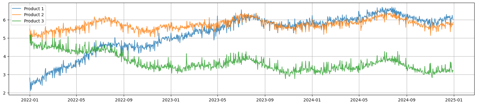
Figure 1a. ln(demand) for each product across time

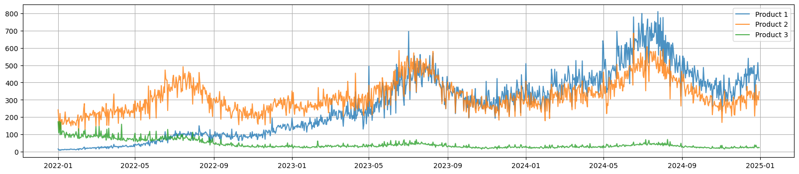
Figure 1b. Demand for each product across time

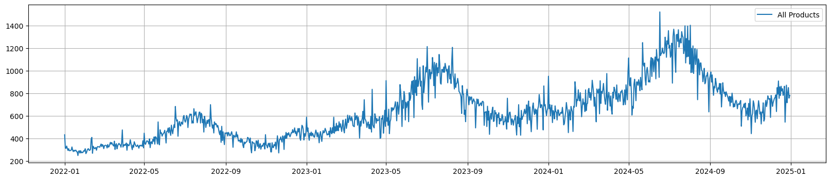
Figure 1c. Total Demand across time

3.2 Visualizing Trend and Seasonality

We can see the different trend and shared seasonality components.

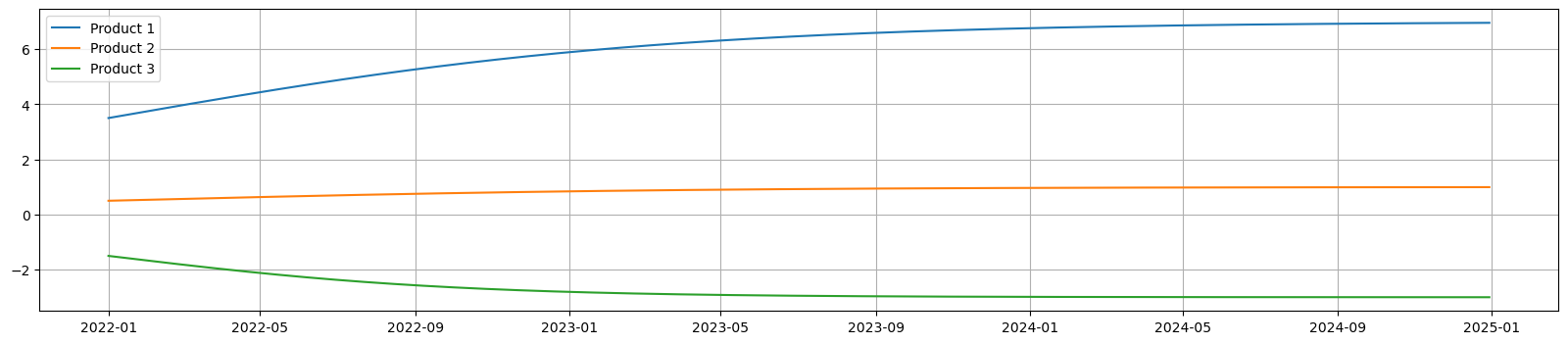
Figure 2a. Trend for each product across time

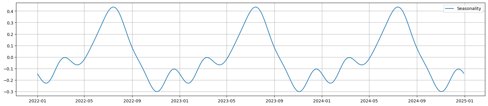
Figure 2b. Monthly Seasonality across time

3.3 Visualizing Price and Elasticities

Lastly, the plots below shows price ranges and their elasticities among the 3 products. Due to random price flucuation and the cross elasticities of products, the association of demand w.r.t. the product's price may not be that obvious, but we can still subtly observe that from the charts.

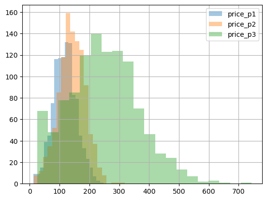
Figure 3a. Price distribution for each product

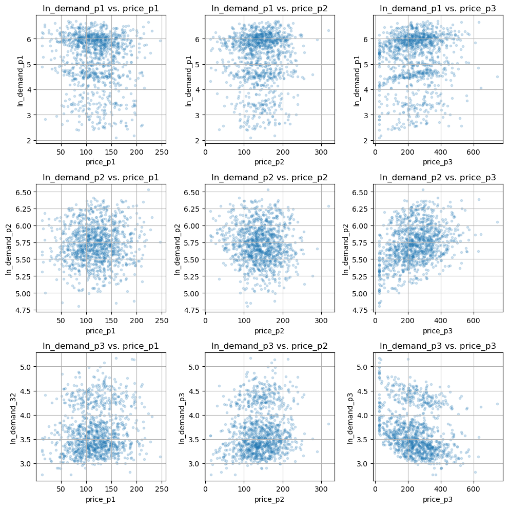
Figure 3b. Price and Cross Elasticities

4. Summary

In summary, I have demonstrated:

how to synthesize a time series dataset that captures both price elasticities and cross elasticities, reflecting closer real-world dynamics between related products
integration of trend (logistic growth), seasonality (Fourier series) into the synthetic data
Python implementation for generating this dataset

In future posts, I'll exploring more in pricing using this dataset, including:

Bayesian frameworks to quantify uncertainty in elasticity estimates of multiple products
Optimizing product portfolio prices for maxmizing revenue or profit

Stay tuned for these applications and more research and experiments!

References:

Taylor, S. J., & Letham, B. (2018). Forecasting at scale. The American Statistician, 72(1), 37–45.