Hyperparameter Tuning using Ray Tune Search Algorithms: Bayesian Optimization and HyperOpt

In my previous post, I have implemented an experiment tracking pipeline that logs the model hyperparameters, validations curves, feature importances, inference data, and most importantly the performance metrics. Right now, we're pretty much geared up to explore and exploit Ray Tune to perform hyperparameter tuning.

In this post, I’ll leverage Ray Tune to perform hyperparameter tuning using Bayesian Optimization and HyperOpt. I will define the search space, implement the algorithms, and compare their performance against manual tuning from the previous post.

1. About Hyperparameter Tuning

Hyperparameters are values to be set to control the learning process of a model, where a model's parameters will be optimized to some objective. Thus the name "hyper" in hyperparameter, it's a meta parameter to tune the model's parameter (e.g. coefficients in a linear regression model). Examples of hyperparameters include the learning rate in gradient-based optimization, the number of layers in a neural network, or the depth of a decision tree.

When models get more complex, from linear regression to gradient boosting machines to deep neural networks, optimizing the hyperparameters to achieve good model performance gets harder and harder. This is because the hyperparameter search space is often vast, non-linear, and noisy with respect to the model's objective function. This makes tuning hyperparameters manually both inefficient and often suboptimal.

# [Manual] MSE: 0.45601, R^2: 0.39781
{
    "learning_rate": 0.001, "max_depth": 8, "subsample": 1.0,
    "colsample_bytree": 1.0, "min_child_samples": 5,
    "reg_alpha": 0.0, "reg_lambda": 0.0,
}

2. Search Algorithms

Search algorithms are a smarter way to explore the hyperparameter space more systematically and effectively, as well as automating the model optimization process. Essentially, search algorithms find some optimal/suboptimal solution to some combinatorial problems like hyperparameter tuning. In the context of hyperparameter tuning, some examples of search algorithms are grid search, random search, bayesian optimization and algorithms based on evolutionary strategies.

Prior to diving into search algorithms further, there is another class of algorithms related to hyperparameter tuning I would like to hightlight — Schedulers. Schedulers manage the allocation of computational resources during the search process, often in a distributed or concurrent training environment. While search algorithms focus on finding optimal model parameters, schedulers determine how search trials are scheduled and executed, when they are terminated if underperforming. For today, I will not be diving into schedulers, but just search algorithms.

I will be making use of the experiment tracking pipeline from my previous post, along with the UCI Wine Quality dataset and the LightGBM algorithm for hyperparameter tuning. I will be exploring the use of Bayesian Optimization and HyperOpt with the following search space for LightGBM model parameters:

search_space = {
    "objective": "regression",
    "n_estimators": 5000,
    "learning_rate": tune.loguniform(1e-4, 1e-2),
    "max_depth": tune.randint(6, 12),
    "subsample": tune.uniform(0.8, 1.0),
    "colsample_bytree": tune.uniform(0.5, 1.0),
    "min_child_samples": tune.randint(2, 10),
    "reg_alpha": tune.uniform(0.0, 1.0),
    "reg_lambda": tune.uniform(4.0, 10.0),
    "n_jobs": 1,  # Make sure to lower n_threads to avoid deadlocks
}

2.1 Bayesian Optimization

Bayesian Optimization is a strategy for optimizing complex, black-box functions that are expensive to evaluate. It uses a simpler function called the surrogate function to approximate the model performance (e.g. MSE, loss, etc...) based on the input set of hyperparameters. The surrogate function used is often a Gaussian Process, which predicts the expected performance and its uncertainty. Given the surrogate function predictions, an acquisition function determines the next hyperparameter set to evaluate. The acquisition function is mainly where exploration and exploitation is controlled, and there are different strategies for this function:

Upper Confidence Bound (UCB) and Lower Confidence Bound (LCB). UCB/LCB prioritize regions with high uncertainty or promising outcomes. UCB is typically used for maximization problems, while LCB is used for minimization. They combine the surrogate model's mean prediction $\mu(x)$ and standard deviation $\sigma(x)$ to form a confidence bound, guiding the search towards areas with potential for improvement.

Expected Improvement (EI). EI focuses on maximizing the expected gain over the current best observation. It calculates the expected amount by which a new evaluation will improve over the best-known value, considering both the predicted mean and uncertainty. This approach balances exploration and exploitation by favoring points that are likely to yield significant improvements.

Probability of Improvement (PI). PI selects configurations with the highest likelihood of outperforming the current best result. It estimates the probability that a new evaluation will exceed the best-known value, focusing on areas with a high chance of improvement. While PI can be effective, it may be less exploratory compared to EI, potentially leading to local optima.

With that understanding, let's implement that in Ray Tune using the UCB approach.

Note: LCB is not implemented in Ray Tune library so I will make some tweaks


def run_ray_tune():
    search_space = {
        "objective": "regression",
        "n_estimators": 5000,
        "learning_rate": tune.loguniform(1e-4, 1e-2),
        "max_depth": tune.uniform(6, 13),
        "subsample": tune.uniform(0.8, 1.0),
        "colsample_bytree": tune.uniform(0.5, 1.0),
        "min_child_samples": tune.uniform(2, 10),
        "reg_alpha": tune.uniform(0.0, 1.0),
        "reg_lambda": tune.uniform(4.0, 10.0),
        "n_jobs": 1,  # Make sure to lower n_threads to avoid deadlocks
    }

    algo = BayesOptSearch(utility_kwargs={"kind": "ucb", "kappa": 4.5, "xi": 0.0})
    algo = ConcurrencyLimiter(algo, max_concurrent=10)

    tuner = tune.Tuner(
        train_lightgbm,
        tune_config=tune.TuneConfig(
            metric="mse",
            mode="max",
            search_alg=algo,
            num_samples=50,  # simulate # of samples of hyperparameter config (bayesopt)
        ),
        param_space=search_space,
    )
    results = tuner.fit()

    print("Best hyperparameters found were: ", results.get_best_result().config)



def train_lightgbm(config):
    config.update({"max_depth": int(config["max_depth"])})
    config.update({"min_child_samples": int(config["min_child_samples"])})

    # Remaining code... (Refer to previous post)
    # ...

    results = {
        # Maximize the negative MSE. (LCB not implemented so we have to do this)
        "mse": sklearn.metrics.mean_squared_error(valid_y, preds) * -1,
        "rmse": sklearn.metrics.mean_squared_error(valid_y, preds) ** 0.5,
        "r2_score": sklearn.metrics.r2_score(valid_y, preds),
    }

    # Remaining code... (Refer to previous post)
    # ...

As Bayesian Optimization requires hyperparameters in the search space to be continuous, we need to sample from some continuous distribution, which does not work on discrete parameters such as max_depth and min_child_samples. To workaround this issue, we can sample from a uniform continuous distribution, convert it into an integer prior to instantiating our model with the hyperparameters. Also, since we can only use UCB and not LCB, I've multipled the MSE by -1 and set the TuneConfig to maximize the negative MSE.

When using UCB as our acqusition function, we can control how much to explore and exploit using the parameter $\kappa$ . Based on Nogueira (2014–), the UCB is calculated simply by:

UCB(x) = \mu(x) + \kappa~\sigma(x)

We see easily that higher values of $\kappa$ results in a larger uncertainty, encouraging the algorithm to explore regions of the search space, while lower values of $\kappa$ results in lower uncertainty, making the algorithm more likely to exploit areas known to have high predicted performance. Selecting an appropriate $\kappa$ value is essential for effective optimization, as it directly impacts the algorithm's ability to discover optimal solutions by balancing the need to explore new possibilities and exploit existing knowledge.

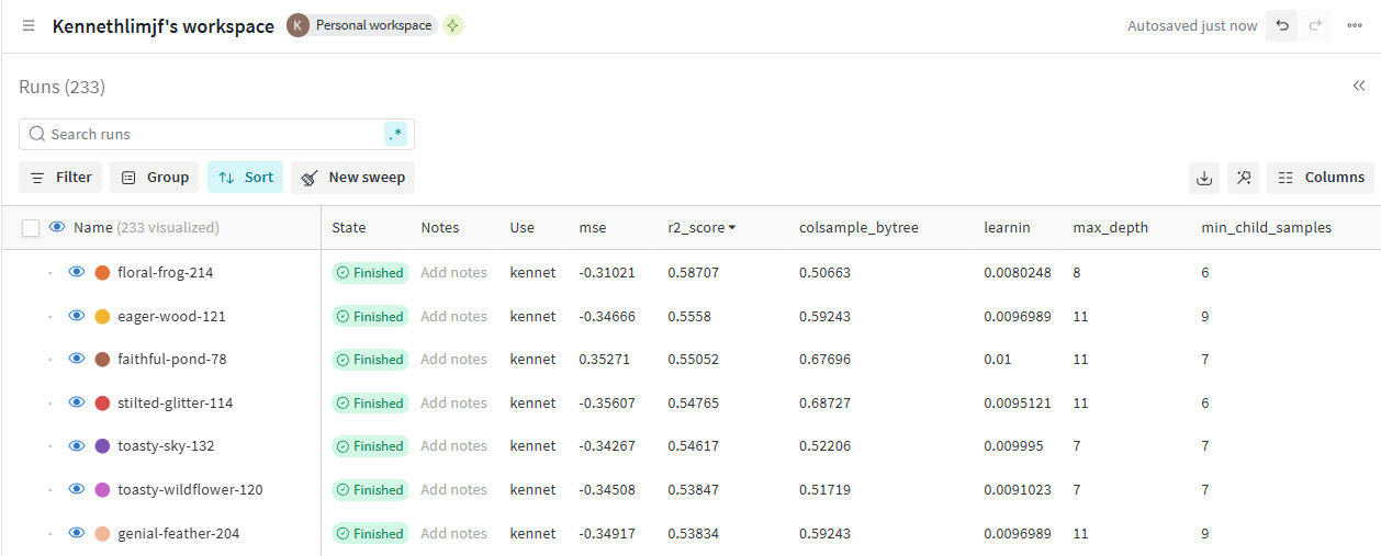
After running multiple experiment trials with different sets of hyperparameters evaluated by Bayesian Optimization, here are the results:

The best result obtained after running a few hundred experiments:

# [BayesOpt] MSE: 0.31021, R^2: 0.58707
{
    "learning_rate": 0.0080248, "max_depth": 8, "subsample": 0.94871,
    "colsample_bytree": 0.50663, "min_child_samples": 6,
    "reg_alpha": 0.47101, "reg_lambda": 5.75695,
}

2.2 HyperOpt

Another search algorithm that is popular is HyperOpt, which is based on the Tree-structured Parzen Estimator (TPE). Previously in Bayesian Optimization, we build a surrogate function $p(y|x)$ to predict the model performance based on a sampled hyperparameter set. On the contrary, TPE models the probabilistic functions that estimates the distributions $p(x|y)$ and $p(y)$ , which is then used to search for promising regions of the hyperparameter space.

Referring to Bergstra et al. (2011), TPE uses two densities to define $p(x|y)$ :

p(x \mid y) = \begin{cases} \ell(x) & \text{if } y < y^*, \\ g(x) & \text{if } y \geq y^*, \end{cases}

The density $l(x)$ represents the likelihood of hyperparameters resulting in objective function values lower than a specified threshold, while $g(x)$ represents the likelihood of hyperparameters resulting in objective function values higher than that threshold. (note: lower loss $y$ is better). The TPE algorithm uses $\gamma$ to be some quantile of the observed losses $y$ such that $P(y \lt y^*) = \gamma$ . TPE employs the EI strategy and calculates the EI proportional to:

EI_{y^*}(x) \propto \bigg( \gamma + \frac{g(x)}{l(x)} (1 - \gamma) \bigg) ^ {-1}

For any given set of hyperparameter $x$ , we can see that a higher probability for $l(x)$ (distribution with better loss) and a lower probability for $g(x)$ is preferred. $\gamma$ here plays a crucial role in the degree of explore-exploit, and 0.25 is often the typical value used. Finally, by modeling the hyperparameters search space hierarchically in a tree structure and using the Parzen Estimator, TPE is able to efficient sample multiple candidates and select the best one with the greatest EI.

Since HyperOpt (Bergstra et al., 2013) is able to handle both discrete and continuous hyperparameters, the implementation is pretty straight-forward, without needing any modification to our training function from the previous post:


def run_ray_tune():
    search_space = {
        "objective": "regression",
        "n_estimators": 5000,
        "learning_rate": tune.loguniform(1e-4, 1e-2),
        "max_depth": tune.randint(6, 12),
        "subsample": tune.uniform(0.8, 1.0),
        "colsample_bytree": tune.uniform(0.5, 1.0),
        "min_child_samples": tune.randint(2, 10),
        "reg_alpha": tune.uniform(0.0, 1.0),
        "reg_lambda": tune.uniform(4.0, 10.0),
        "n_jobs": 1,  # Make sure to lower n_threads to avoid deadlocks
    }

    algo = HyperOptSearch(n_initial_points=50)
    algo = ConcurrencyLimiter(algo, max_concurrent=20)

    tuner = tune.Tuner(
        train_lightgbm,
        tune_config=tune.TuneConfig(
            metric="mse",
            mode="min",
            search_alg=algo,
            num_samples=150  # simulate # of samples of hyperparameter config (bayesopt)
        ),
        param_space=search_space,
    )
    results = tuner.fit()

    print("Best hyperparameters found were: ", results.get_best_result().config)

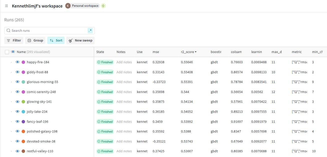
After running multiple experiment trials with different sets of hyperparameters evaluated by HyperOpt, here are the results:

The best result obtained after running a few hundred experiments using HyperOpt:

# [HyperOpt] MSE: 0.32938, R^2: 0.55646
{
    "learning_rate": 0.0069488, "max_depth": 11, "subsample": 0.85587,
    "colsample_bytree": 0.76603, "min_child_samples": 3,
    "reg_alpha": 0.64303, "reg_lambda": 5.12598,
}

3. Summary

In this post, we explored two advanced hyperparameter tuning algorithms—Bayesian Optimization and HyperOpt—and compared their performance to manual tuning.

Both methods demonstrated significant improvements over the manual tuning process in efficiency and model performance. The best performing model was found using Bayesian Optimization, and there may be a few explanations for this.

It could be possible that modelling of $P(y|x)$ is more accurate than $P(x|y)$ resulting in better estimation and selection of potential candidates.
We employed different acqusition strategies and it could be that UCB had a better exploration and exploitation trade-off, resulting in finding a better set of hyperparameters

Nevertheless, we should always experiment with all sorts of methods and strategies to find the best model because we know there is no free lunch in machine learning.

Thanks for reading this post and I hope you enjoyed this one!

References:

Bergstra, J., Bardenet, R., Bengio, Y., & Kégl, B. (2011). Algorithms for Hyper-Parameter Optimization. In J. Shawe-Taylor, R. Zemel, P. Bartlett, F. Pereira, & K. Q. Weinberger (Eds.), Advances in Neural Information Processing Systems (Vol. 24). Curran Associates, Inc. https://proceedings.neurips.cc/paper_files/paper/2011/file/86e8f7ab32cfd12577bc2619bc635690-Paper.pdf

Bergstra, J., Yamins, D., & Cox, D. (2013). Making a Science of Model Search: Hyperparameter Optimization in Hundreds of Dimensions for Vision Architectures. In S. Dasgupta & D. McAllester (Eds.), Proceedings of the 30th International Conference on Machine Learning (Vol. 28, Issue 1, pp. 115–123). PMLR. https://proceedings.mlr.press/v28/bergstra13.html

Nogueira, F. (2014–). Bayesian Optimization: Open source constrained global optimization tool for Python. %20https://github.com/bayesian-optimization/BayesianOptimization