Modeling Via Synthesizing Data. And Vice Versa

Scientists have great imagination. Combined with observations, scientists create hypotheses, reason with logic, and create simple mental models that can explain certain phenomenon in our world. As a data scientist, I felt that the process of synthesizing data can really benefit us to become better thinkers, reasoners, problem solvers, and contributors to our society.

In this post, I attempt to synthesize a dataset that can be used to model price elasticity. The dataset will be a time series of demand affected by features such as month, day of week, holiday, and price. Subsequently in my future posts, I will be using this dataset to explore different models for estimating price elasticity of demand and benchmarking.

An overview, I will start from a simple base demand model, and add various features along the way.

Base Demand Model

First, consider the simplest base model with base demand $\alpha$ and noise:

ln(Q_t) = \alpha + \epsilon_t

where:

$\alpha$ is the constant that represents the log of base demand
$\epsilon_t$ is the error term

def generate_dataset(n_days, alpha, err_std):
    date = pd.date_range(start='2022-01-01', periods=n_days, freq='D')

    epsilon = np.random.normal(0, err_std, size=n_days)
    demand = np.exp(alpha + epsilon)

    data = pd.DataFrame({
      'date': date,
      'demand': demand,
    })
    return data

df = generate_dataset(
    n_days=365 * 2,
    alpha=5.5,
    err_std=0.002,
)

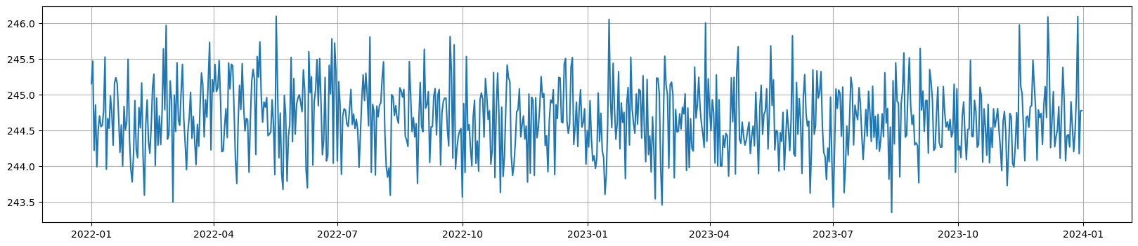
Figure 1. Base Demand Model

Add Linear Trend

Next, we can add a linear trend to the base model to mimic some modest growth in demand over time, by revising our function like this:

ln(Q_t) = \alpha \;+\; \phi T_t \;+\; \epsilon_t

where the new terms:

$\phi$ is the effect for the trend $T_t$
$T_t$ is a simple time index e.g. $T_1 = 1, T_2 = 2, ...$

def generate_dataset(n_days, alpha, err_std, phi):
    date = pd.date_range(start='2022-01-01', periods=n_days, freq='D')

    epsilon = np.random.normal(0, err_std, size=n_days)
    trend = np.arange(n_days) * phi
    demand = np.exp(
        alpha
        + trend
        + epsilon
    )

    data = pd.DataFrame({
        'date': date,
        'demand': demand,
    })
    return data

df = generate_dataset(
    n_days=365 * 2,
    alpha=5.5,
    err_std=0.002,
    phi=1e-4,
)

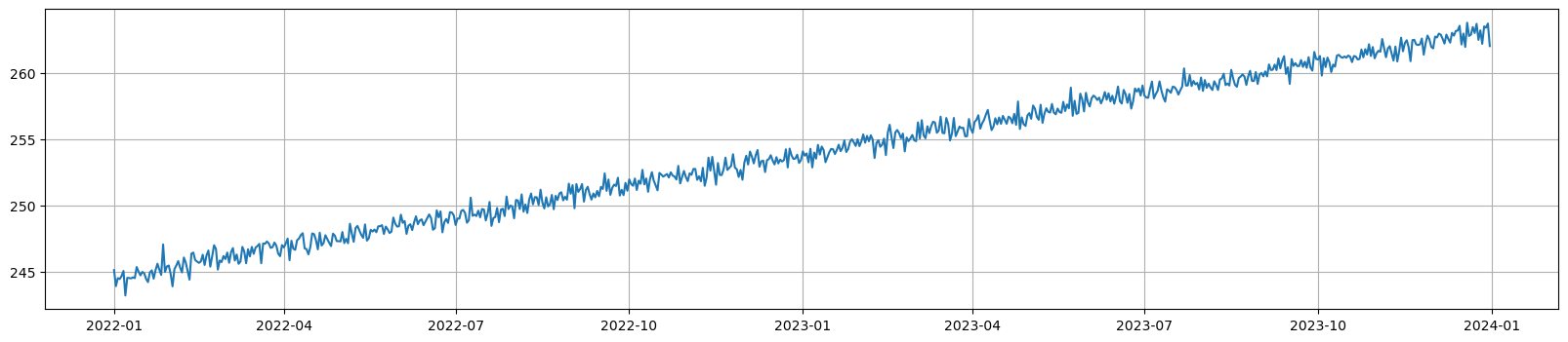
Figure 2. Add Linear Trend

Add Month and Day-of-Week Seasonality

To make it more realistic, we can add month and day-of-week seasonality. Consumers may like to shop more at the mid-year, end-of-year and preferably on weekends.

ln(Q_t) = \alpha \;+\; \sum_{m=1}^{12} \gamma_m \, M_{t,m} \;+\; \sum_{d=1}^{7} \delta_d \, D_{t,d} \;+\; \phi T_t \;+\; \epsilon_t

where the new terms:

$\gamma_{m}$ represents the effect for each of month $m$ , and $M_{t,m}$ = 1 if $t$ is in that month
$\delta_{d}$ represents the effect for each of day of week $m$ , and $D_{t,d}$ = 1 if $t$ is in that day of week
$M_{t,m}, D_{t,d}$ are month, day-of-week dummy variables respectively

def generate_dataset(n_days, alpha, err_std, phi, gamma, delta):
    date = pd.date_range(start='2022-01-01', periods=n_days, freq='D')

    # Monthly seasonality
    df_months = pd.DataFrame({ "month": [d.month for d in date] })
    M = pd.get_dummies(df_months, columns=["month"], prefix="M").astype(int).values
    seasonality_month = (M @ gamma.reshape(-1, 1)).ravel()

    # Day of week seasonality
    df_dow = pd.DataFrame({ "dow": [d.dayofweek for d in date] })
    D = pd.get_dummies(df_dow, columns=["dow"], prefix="D").astype(int).values
    seasonality_dow = (D @ delta.reshape(-1, 1)).ravel()

    # Trend
    trend = np.arange(n_days) * phi

    # Error
    epsilon = np.random.normal(0, err_std, size=n_days)

    demand = np.exp(
        alpha
        + seasonality_month
        + seasonality_dow
        + trend
        + epsilon
    )

    data = pd.DataFrame({
        'date': date,
        'demand': demand,
    })
    return data

df = generate_dataset(
    n_days=365 * 2,
    alpha=5.5,
    err_std=0.002,
    phi=1e-4,
    gamma=np.array([
        0.01, -0.01, 0.0,
        0.02, 0.03, 0.04,
        0.03, 0.01, -0.03,
        -0.01, 0.0, 0.02
    ]),
    delta=np.array([0.0, -0.02, 0.01, 0.0, 0.02, 0.01, 0.0])
)

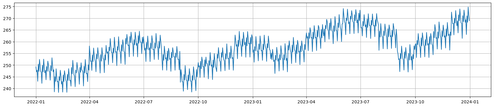
Figure 3. Add Seasonality

Add Holiday

Holiday events are often important in most time series forecasts as demand spikes are often caused by these events. To include this, we'll need a holiday calendar.

holiday_dict = {
    "New Year Day": [(1, 1)],
    "Chinese New Year": [(10, 2), (11, 2)],
    "Good Friday": [(29, 3)],
    "Hari Raya Puasa": [(10, 4)],
    "Labour Day": [(1, 5)],
    "Vesak Day": [(22, 5)],
    "Hari Raya Haji": [(17, 6)],
    "National Day": [(9, 8)],
    "Deepavali": [(31, 10)],
    "Christmas Day": [(25, 12)],
}

holiday_dates = [t for l in holiday_dict.values() for t in l]

def generate_dataset(n_days, alpha, err_std, phi, gamma, delta, theta, holiday_dates):
    date = pd.date_range(start='2022-01-01', periods=n_days, freq='D')

    # Holiday
    def _is_holiday(d, holiday_dates):
        if (d.day, d.month) in holiday_dates:
            return 1
        return 0

    holiday = np.array([_is_holiday(d, holiday_dates) * theta for d in date])

    # Monthly seasonality
    df_months = pd.DataFrame({ "month": [d.month for d in date] })
    M = pd.get_dummies(df_months, columns=["month"], prefix="M").astype(int).values
    seasonality_month = (M @ gamma.reshape(-1, 1)).ravel()

    # Day of week seasonality
    df_dow = pd.DataFrame({ "dow": [d.dayofweek for d in date] })
    D = pd.get_dummies(df_dow, columns=["dow"], prefix="D").astype(int).values
    seasonality_dow = (D @ delta.reshape(-1, 1)).ravel()

    # Trend
    trend = np.arange(n_days) * phi

    # Error
    epsilon = np.random.normal(0, err_std, size=n_days)

    demand = np.exp(
        alpha
        + seasonality_month
        + seasonality_dow
        + trend
        + holiday
        + epsilon
    )

    data = pd.DataFrame({
      'date': date,
      'demand': demand,
    })
    return data

df = generate_dataset(
    n_days=365 * 2,
    alpha=5.5,
    err_std=0.002,
    phi=1e-4,
    gamma=np.array([
      0.01, -0.01, 0.0,
      0.02, 0.03, 0.04,
      0.03, 0.01, -0.03,
      -0.01, 0.0, 0.02
    ]),
    delta=np.array([0.0, -0.02, 0.01, 0.0, 0.02, 0.01, 0.0]),
    theta=0.08,
    holiday_dates=holiday_dates,
)

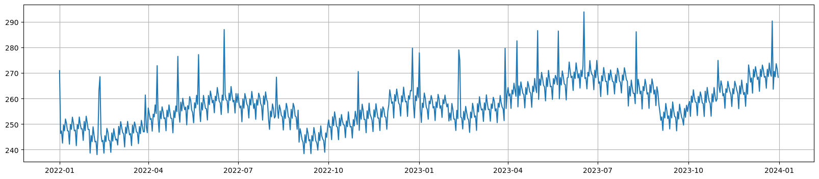
Figure 4. Add Holiday

Add Price Elasticity of Demand

Finally, consider the popular log-log model for price elasticity of demand. The full equation (I think this is sufficient for now, let's stop here):

ln(Q_{t}) = \alpha \;+\; \sum_{m=2}^{12} \gamma_m \, M_{t,m} \;+\; \sum_{d=2}^{7} \delta_d \, D_{t,d} \;+\; \phi T_t \;+\; \theta H_t \;+\; \beta ln(P_t) \;+\; \epsilon_t

where:

$\alpha$ is the constant that represents the log of base demand
$\gamma_{m}$ represents the effect for each of month $m$ , and $M_{t,m}$ = 1 if $t$ is in that month
$\delta_{d}$ represents the effect for each of day of week $m$ , and $D_{t,d}$ = 1 if $t$ is in that day of week
$\theta$ is the effect for holiday if $t$ is a holiday
$M_{t,m}, D_{t,d}, H_t$ are month, day-of-week, and holiday dummy variables respectively
$\phi$ is the effect for the trend $T_t$
$T_t$ is a simple time index e.g. $T_1 = 1, T_2 = 2, ...$
$\beta$ is the price elasticity of demand
$\epsilon_t$ is the error term
$P_t$ is the price for observation $t$

$\beta$ is the price elasticity of demand as we have been taught in our Economics 101 class, which is equivalent to $\frac{\% \, change \, in \, demand}{\% \, change \, in \, price}$ . To write a python function to generate the data based on this equation:

def generate_dataset(n_days, alpha, err_std, phi, gamma, delta, theta, holiday_dates, beta, price_mean, price_std):
    date = pd.date_range(start='2022-01-01', periods=n_days, freq='D')

    # Holiday
    def _is_holiday(d, holiday_dates):
        if (d.day, d.month) in holiday_dates:
            return 1
        return 0

    H = np.array([_is_holiday(d, holiday_dates) for d in date]).astype(int)
    holiday = H * theta

    # Monthly seasonality
    df_months = pd.DataFrame({ "month": [d.month for d in date] })
    M = pd.get_dummies(df_months, columns=["month"], prefix="M").astype(int)
    seasonality_month = (M.values @ gamma.reshape(-1, 1)).ravel()

    # Day of week seasonality
    df_dow = pd.DataFrame({ "dow": [d.dayofweek for d in date] })
    D = pd.get_dummies(df_dow, columns=["dow"], prefix="D").astype(int)
    seasonality_dow = (D.values @ delta.reshape(-1, 1)).ravel()

    # Trend
    T = np.arange(n_days)
    trend = T * phi

    # Price Elasticity of demand
    price = np.round(
        np.clip(
            np.random.normal(price_mean, price_std, size=n_days),
            0.2 * price_mean,
            3.0 * price_mean
        ), 2
    )
    q = beta * np.log(price)

    # Error
    epsilon = np.random.normal(0, err_std, size=n_days)

    demand = np.exp(
        alpha
        + seasonality_month
        + seasonality_dow
        + trend
        + holiday
        + q
        + epsilon
    ).astype(int)

    data = pd.DataFrame({
        'date': date,
        'H_t': H,
        'T_t': T,
        'demand': demand,
        'price': price,
        'd_q': q,
    })

    return pd.concat([
      data,
      D,
      M,
    ], axis=1)

df = generate_dataset(
    n_days=365 * 5,
    alpha=5.8,
    err_std=0.03,
    phi=1e-4,
    gamma=np.array([
      0.01, -0.01, 0.0,
      0.02, 0.03, 0.04,
      0.03, 0.01, -0.03,
      -0.01, 0.0, 0.02
    ]),
    delta=np.array([0.0, -0.02, 0.01, 0.0, 0.02, 0.01, 0.0]),
    theta=0.08,
    holiday_dates=holiday_dates,
    beta=-0.06,
    price_mean=80,
    price_std=40,
)

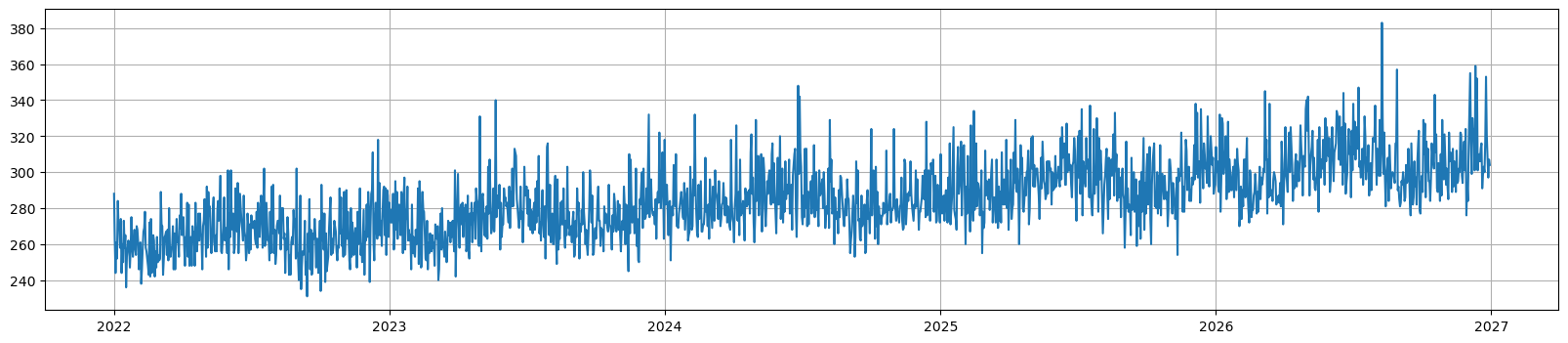
Figure 5. Add Price Elasticity of Demand

We can plot the price elastcity curve to see that as price decreases, the demand increases exponentially.

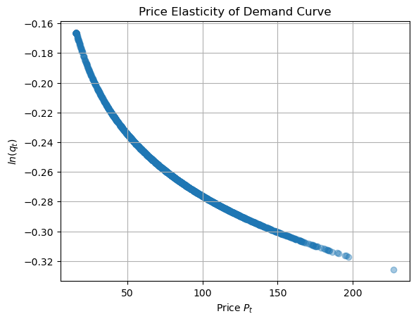
Figure 6. Price Elasticity of Demand

Summary

With this, we've completed the data synthesize process. In summary, we have modeled mainly using simple dummy variables, some linear relations, and a power relation for price. Though this is relatively simple, what's more important is how we go about thinking:

how these explanatory variables are layered one over another?
what the relation of explanatory variables should be with the target variable? or
how explanatory variables affect one another?
what the flow should be like? does the linear model suffice?
if a parametric function is not sufficient to model that relation, can I use a non-parametric function instead?

There are other topics such as Causal Graphs, Structural Equation Models can provide a more robust modeling framework that also addresses causal relations.

But for now, I hope you enjoy reading this post! Have a nice day!